Well I am very ancient for certain but not sure what that has to do with it. Your tone implies that the Smith chart is ancient technology with little place in modern engineering. While it is true that engineers no longer solve problems by plotting points on paper Smith charts or using Smith chart 'slide rules' (I jhave one - it belonged to my father) all good modern network analyzers have a Smith chart display and a good engineer knows how to read it. While return loss is valuable information it gives no hint as to what the cause is. A Smith chart does that at a glance.Wow smith chart? how old are you? lol I saw smith chart I think in Tech college and never saw it again! hahaha.... Answer is no I dont have a smith chart sorry bud!

5.8 antenna
- Thread starter indonesianpilot
- Start date
-
- Tags
- antenna ghz
You are using an out of date browser. It may not display this or other websites correctly.
You should upgrade or use an alternative browser.
You should upgrade or use an alternative browser.
Well I am very ancient for certain but not sure what that has to do with it. Your tone implies that the Smith chart is ancient technology with little place in modern engineering. While it is true that engineers no longer solve problems by plotting points on paper Smith charts or using Smith chart 'slide rules' (I jhave one - it belonged to my father) all good modern network analyzers have a Smith chart display and a good engineer knows how to read it. While return loss is valuable information it gives no hint as to what the cause is. A Smith chart does that at a glance.
HAHA no no dont take it the wrong way bud! My service monitor at work that I use about 3 times a week has the smith chart view on it, but i never use it HAHAH!! We just dont need to go that deep! But yes you are correct in saying that it gives more detailed plots for sure!!
") Have a goo day!
Have a goo day!After thinking about Smith charts I'd like to change my answer here. First thing is test to see whether I can get an image in here. I guess I can so, OK here goes. You can't really convert the antenna itself but you can 'match' it to the transmitter/receiver. Assuming you had a network analyzer available to scan a 5.8 antenna at 2.4 GHz the antenna would appear on a Smith chart display somewhere like where the blue dot is on the attached picture. This is a terrible match with the antenna radiation resistance being about (multiply all numbers by 50) .09 (you want 1) with a reactive component of about -0.2 (you want 0). This results in a VSWR of 12.7:1 (terrible) and a return loss of -1.37 db. Most of the power delivered to this antenna will be reflected back to the transmitter.Is there any way to convert 5.8 antenna to 2.4?
To match move the blue dot along the dashed line circle (counterclock wise) until you hit the green circle. This is easily done by connecting a short (about 0.15 wavelength) piece of transmission line (coax) to the antenna. The green circle is the locus of points with conductance equal 1 (G = 1) so the conductance looking in to the other end of that coax is G = 1. The blue dot, before and after moving it represents impedance and the reactive impedance of the moved dot is about -2.8j (it is close to the -0.3 line and the j denotes it as a reactance). We could cancel it by putting a reactance of + 2.8j in series with the short piece of cable. A capacitor of 1/(2*pi*2.4E-3*2.8*50) = 0.47pf would do but that's pretty small so we look at another approach and that is to convert the impedance at the shifted point to the admittance at that point and this is done by reflecting the shifted point along the straight line through the center of the diagram until the heavy red unit circle is met on the other side. The admittance at this point is Y = 1 + 3.5j (1 because the red circle is the G=1 circle and 3.5 is obtained by eyeballing the distance along the arc between the 3 and 5 curves. If we add a conductance G' = 0 - 3.5 j in parallel at the input to the short cable end (effectively moving along the G=1 circle towards the origin we get G'' = 1 + 0j, the intersection of the heavy red line and heavy red circle. An easy and convenient way to obtain a conductance of 0 - 3.5j is by taking another piece of transmission line shorted at one end. To see how long this should be we plot -3.5j on the outer circle of the diagram and project that thru the center to see where it hits the other side or just calculate 1/-3.5j = 0.29j (j is a rather special number such that 1/j = -j) which says that j*j = -1) and plot that on the outer circle where the pencil dot is in the picture. Starting at where the heavy red lone intersects this outer circle (9 o'clock) and rotating clockwise until the pencil dot is reached you will go 9% of the way around the circle. Since once around the circle corresponds to two wavelengths we find that we need 4.5% of a wavelength of cable to put in parallel with the first piece of cable. This is what devices like the 'tee' pictured in #11 are for. The input to the third leg on the tee is G = 1 + j0 and the reciprocal of that is the impedance Z = 1 + j0. Un-normalizing by multiplying by 50 we have Zs = 50 + j0 Ω - a perfect match.
So conceptually you could build a matching network for that 5 GHz antenna and get it on the air. It probably wouldn't be practical to do it with coax as the pieces would be so short but it could be done with strip line. The real purpose of this is to illustrate the ease with which matching problems can be solved if one has the Smith chart to look at.
Attachments
Last edited:
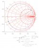
After thinking about Smith charts I'd like to change my answer here. First thing is test to see whether I can get an image in here. I guess I can so, OK here goes. You can't really convert the antenna itself but you can 'match' it to the transmitter/receiver. Assuming you had a network analyzer available to scan a 5.8 antenna at 2.4 GHz the antenna would appear on a Smith chart display somewhere like where the blue dot is on the attached picture. This is a terrible match with the antenna radiation resistance being about (multiply all numbers by 50) .09 (you want 1) with a reactive component of about -0.2 (you want 0). This results in a VSWR of 12.7:1 (terrible) and a return loss of -1.37 db. Most of the power delivered to this antenna will be reflected back to the transmitter.
To match move the blue dot along the dashed line circle (counterclock wise) until you hit the green circle. This is easily done by connecting a short (about 0.15 wavelength) piece of transmission line (coax) to the antenna. The green circle is the locus of points with conductance equal 1 (G = 1) so the conductance looking in to the other end of that coax is G = 1. The blue dot, before and after moving it represents impedance and the reactive impedance of the moved dot is about -2.8j (it is close to the -0.3 line and the j denotes it as a reactance). We could cancel it by putting a reactance of + 2.8j in series with the short piece of cable. A capacitor of 1/(2*pi*2.4E-3*2.8*50) = 0.47pf would do but that's pretty small so we look at another approach and that is to convert the impedance at the shifted point to the admittance at that point and this is done by reflecting the shifted point along the straight line through the center of the diagram until the heavy red unit circle is met on the other side. The admittance at this point is Y = 1 + 3.5j (1 because the red circle is the G=1 circle and 3.5 is obtained by eyeballing the distance along the arc between the 3 and 5 curves. If we add a conductance G' = 0 - 3.5 j in parallel at the input to the short cable end (effectively moving along the G=1 circle towards the origin we get G'' = 1 + 0j, the intersection of the heavy red line and heavy red circle. An easy and convenient way to obtain a conductance of 0 - 3.5j is by taking another piece of transmission line shorted at one end. To see how long this should be we plot -3.5j on the outer circle of the diagram and project that thru the center to see where it hits the other side or just calculate 1/-3.5j = 0.29j (j is a rather special number such that 1/j = -j) which says that j*j = -1) and plot that on the outer circle where the pencil dot is in the picture. Starting at where the heavy red lone intersects this outer circle (9 o'clock) and rotating clockwise until the pencil dot is reached you will go 9% of the way around the circle. Since once around the circle corresponds to two wavelengths we find that we need 4.5% of a wavelength of cable to put in parallel with the first piece of cable. This is what devices like the 'tee' pictured in #11 are for. The input to the third leg on the tee is G = 1 + j0 and the reciprocal of that is the impedance Z = 1 + j0. Un-normalizing by multiplying by 50 we have Zs = 50 + j0 Ω - a perfect match.
So conceptually you could build a matching network for that 5 GHz antenna and get it on the air. It probably wouldn't be practical to do it with coax as the pieces would be so short but it could be done with strip line. The real purpose of this is to illustrate the ease with which matching problems can be solved if one has the Smith chart to look at.
LOL over most peoples heads in here man! To be honest I didn't read the whole thing. But seems most accurate. I myself will just sweep them using VSWR/Return loss. Way easier to understand and follow. I would like to sweep some of those alpha panel antennas... maybe i will buy some and sweep them? Havn't decided yet, I think i want new props first haha.
I didn't expect anyone to follow completely and I simplified stuff a lot because all I really wanted do was make people aware that Smith chart may offer things you weren't aware of and that might actually be useful to to at some time in the future (or present). For example, the distance for the center of the plot to the blue dot + 1 divided by distance - 1 is the VSWR. -20 log(distance) is the return loss.
Now if you do happen to sweep some of the after market antennas in return loss mode and wouldn't mind grabbing a sweep in Smith mode (hint, hint)....
Now if you do happen to sweep some of the after market antennas in return loss mode and wouldn't mind grabbing a sweep in Smith mode (hint, hint)....

as far as i understand electricity,then : its true that electrons have to travel into the circuit and make a successful exit out of the circuit in order for that circuit to work. right ? (a short circuit means the flow didnt make it out) and radio signals are electrons, yes ? an antenna has 2 connections true ? the signal (or center wire) and the "ground" as it called. does the theory of elecrton flow hold true in this application ? the signak goes in thru the center lead and exits the device thru the ground right ? where do those electrons go ? they cant go out as a transmission ,wouldnt that cause mega interference i was also told electrons we make never just die or were they just a-foolin ? just askin
- Joined
- Mar 12, 2016
- Messages
- 3,920
- Reaction score
- 2,626
Are you on drugs? Just askin.as far as i understand electricity,then : its true that electrons have to travel into the circuit and make a successful exit out of the circuit in order for that circuit to work. right ? (a short circuit means the flow didnt make it out) and radio signals are electrons, yes ? an antenna has 2 connections true ? the signal (or center wire) and the "ground" as it called. does the theory of elecrton flow hold true in this application ? the signak goes in thru the center lead and exits the device thru the ground right ? where do those electrons go ? they cant go out as a transmission ,wouldnt that cause mega interference i was also told electrons we make never just die or were they just a-foolin ? just askin
- Joined
- Mar 12, 2016
- Messages
- 3,920
- Reaction score
- 2,626
Nope. It would have been better to lie and admit you were high on something when writing whatever that is you wrote. But ok, I'll humor you. Your understanding of basically everything related to electricity and RF is incorrect.
You mean like AC ?so youre telling me that if electricity doesnt make a full pass in and out of a circuit it still works ? dude youre the one on drugs
same thing with direct current Marconi. Thats why there is a positive and a negative contact on a power supply thats dc. check out electrical theory to find out that if the current(who ever applied)(ac/dc) if the electricity DOES NOT FLOW INTO THE DEVICE BEING POWERED THEN SAID DEVICE SHALL NOT FUNCTION. thats why when something burns out the electricity cannot flow because something has caused a "short circuit" thus preventing said flow of electrons thru device and about that ac comment..in America our alternating current system runs at 60hz. translated that meand 60 time per second the poles change polarity (p to n n to p p to n n to p) but thats because the electrons must pass through the device fully so 60 times a second anything running on ac takes in voltage and shoots it back out thru the n terminal read that last part about flow
Circuits
In order to flow, current electricity requires a circuit: a closed, never-ending loop of conductive material. A circuit could be as simple as a conductive wire connected end-to-end, but useful circuits usually contain a mix of wire and other components which control the flow of electricity. The only rule when it comes to making circuits is they can’t have any insulating gaps in them.
If you have a wire full of copper atoms and want to induce a flow of electrons through it, all free electrons need somewhere to flow in the same general direction. Copper is a great conductor, perfect for making charges flow. If a circuit of copper wire is broken, the charges can’t flow through the air, which will also prevent any of the charges toward the middle from going anywhere.
Last edited:
- Joined
- Mar 12, 2016
- Messages
- 3,920
- Reaction score
- 2,626
yeah i agree. nothing like posting a legit question only to have it trounced by someone whom doesnt even understand theory of electricity.Wow. I opened my 3dr pilot app and this thread was first. There's no need for this people.
I haven't been on this forum in months and this is the first thing I read.
- Joined
- Mar 12, 2016
- Messages
- 3,920
- Reaction score
- 2,626
lol. Have you found anyone in this thread that agrees with anything you've posted? (rhetorical question, the answer is actually no). That may be a indication you're not going down the right road. Or perhaps everyone in the world that's been designing and building antennas forever got it wrong and you've just now discovered the way it should be based on something someone told you about something somewhere.
It may work fine as is. The frequency indicates that the 5.8 is twice the length of the 2.4, so, its' a half wavlwngthAfter thinking about Smith charts I'd like to change my answer here. First thing is test to see whether I can get an image in here. I guess I can so, OK here goes. You can't really convert the antenna itself but you can 'match' it to the transmitter/receiver. Assuming you had a network analyzer available to scan a 5.8 antenna at 2.4 GHz the antenna would appear on a Smith chart display somewhere like where the blue dot is on the attached picture. This is a terrible match with the antenna radiation resistance being about (multiply all numbers by 50) .09 (you want 1) with a reactive component of about -0.2 (you want 0). This results in a VSWR of 12.7:1 (terrible) and a return loss of -1.37 db. Most of the power delivered to this antenna will be reflected back to the transmitter.
To match move the blue dot along the dashed line circle (counterclock wise) until you hit the green circle. This is easily done by connecting a short (about 0.15 wavelength) piece of transmission line (coax) to the antenna. The green circle is the locus of points with conductance equal 1 (G = 1) so the conductance looking in to the other end of that coax is G = 1. The blue dot, before and after moving it represents impedance and the reactive impedance of the moved dot is about -2.8j (it is close to the -0.3 line and the j denotes it as a reactance). We could cancel it by putting a reactance of + 2.8j in series with the short piece of cable. A capacitor of 1/(2*pi*2.4E-3*2.8*50) = 0.47pf would do but that's pretty small so we look at another approach and that is to convert the impedance at the shifted point to the admittance at that point and this is done by reflecting the shifted point along the straight line through the center of the diagram until the heavy red unit circle is met on the other side. The admittance at this point is Y = 1 + 3.5j (1 because the red circle is the G=1 circle and 3.5 is obtained by eyeballing the distance along the arc between the 3 and 5 curves. If we add a conductance G' = 0 - 3.5 j in parallel at the input to the short cable end (effectively moving along the G=1 circle towards the origin we get G'' = 1 + 0j, the intersection of the heavy red line and heavy red circle. An easy and convenient way to obtain a conductance of 0 - 3.5j is by taking another piece of transmission line shorted at one end. To see how long this should be we plot -3.5j on the outer circle of the diagram and project that thru the center to see where it hits the other side or just calculate 1/-3.5j = 0.29j (j is a rather special number such that 1/j = -j) which says that j*j = -1) and plot that on the outer circle where the pencil dot is in the picture. Starting at where the heavy red lone intersects this outer circle (9 o'clock) and rotating clockwise until the pencil dot is reached you will go 9% of the way around the circle. Since once around the circle corresponds to two wavelengths we find that we need 4.5% of a wavelength of cable to put in parallel with the first piece of cable. This is what devices like the 'tee' pictured in #11 are for. The input to the third leg on the tee is G = 1 + j0 and the reciprocal of that is the impedance Z = 1 + j0. Un-normalizing by multiplying by 50 we have Zs = 50 + j0 Ω - a perfect match.
So conceptually you could build a matching network for that 5 GHz antenna and get it on the air. It probably wouldn't be practical to do it with coax as the pieces would be so short but it could be done with strip line. The real purpose of this is to illustrate the ease with which matching problems can be solved if one has the Smith chart to look at.
Its a half wave length, so it will resonate.Well I am very ancient for certain but not sure what that has to do with it. Your tone implies that the Smith chart is ancient technology with little place in modern engineering. While it is true that engineers no longer solve problems by plotting points on paper Smith charts or using Smith chart 'slide rules' (I jhave one - it belonged to my father) all good modern network analyzers have a Smith chart display and a good engineer knows how to read it. While return loss is valuable information it gives no hint as to what the cause is. A Smith chart does that at a glance.
Similar threads
- Replies
- 2
- Views
- 604
- Replies
- 0
- Views
- 1K
New Posts
-
 Free Music / SFX Resource for Your Videos - Over 2000 Tracks
- Latest: Eric Matyas
-
-
-
